Examples
Here are some examples.
1. Ideal PSA simulation for green hydrogen production
In this example, pyAPEP.simide is used to simulate ideal PSA process for the separation of H2/N2 from the green ammonia.
Background
Because green ammonia is currently the favored transportation medium for carbon-free hydrogen, H2 separation and purification technologies have gained increasing attention. Among the various options for H2 separation, pressure swing adsorption (PSA) has the highest technological readiness level. Therefore, this example handle the ideal PSA simulation to produce H2 decomposed from green NH3 and determine the hydrogen recovery of the columns given adsobents properties.
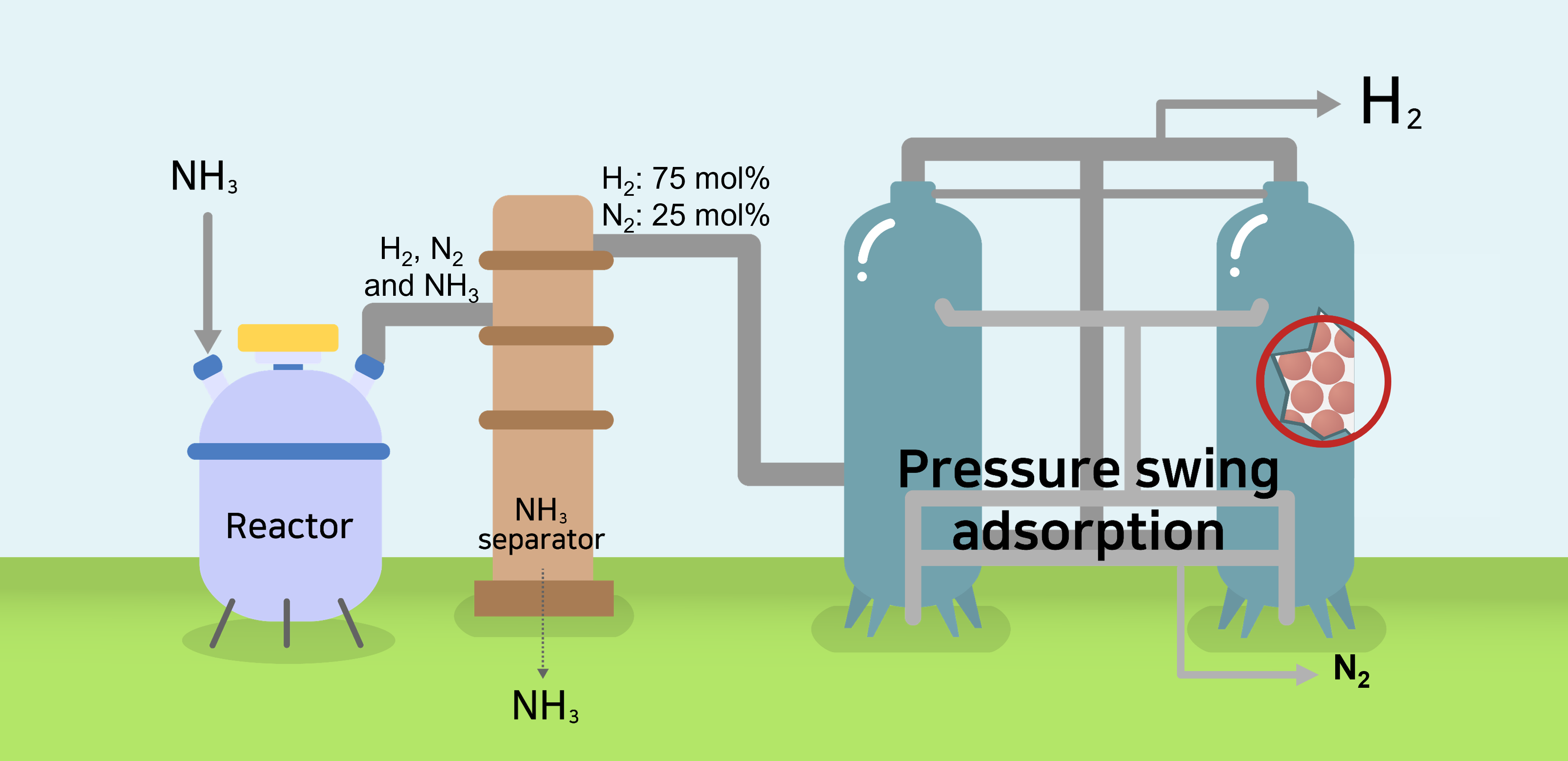
Figure. Schematic of pressure swing adsorption process used for H2 purification.
Process description
H2 produced in regions rich in renewable energy is transported to other locations in the form of NH3, and H2 is produced by decomposing NH3 into a mixture of N2 and H2. The NH3 reactor and residual NH3 removal system are located before the PSA system. Thereafter, the 0.25% of unreacted NH3 exiting the reactor is cooled and removed with a batch type uni-bed adsorption tower. Therefore, the gas entering the target PSA process was assumed to be 25 mol% N2 and 75 mol% H2.
Goal
The goal of this example is the find best adsorbent among three adsorbents by comparing PSA perfomances. Adsorbent candidates are Zeolite 13X, 5A and activated carbon. All adsorbents and its pressure-uptake data could be found in literatures. This example contains isotherm fitting with given data(.csv), isotherm validation, development of mixture isotherm for each adsorbent, and ideal PSA simulation.
Before we start, import pyAPEP package and other python packages for data treatment and visualization. Also, users need to download the adsorption data files for three adsobents
# pyAPEP package import
import pyAPEP.isofit as isofit
import pyAPEP.simide as simide

# Data treatment package import
import numpy as np
import pandas as pd

# Data visualization package import
import matplotlib.pyplot as plt
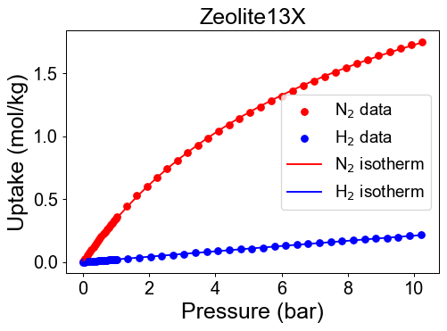
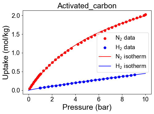
Then, define pure isotherm function for hydrogen and nitrogen using pressure-uptake data samples. Before developing isotherm, users need to define or import datasets. If the isotherm parameters already exist, users can use those parameters by defining isotherm function manually.
#### Data import ####
# adsorbent 1: Zeolite 13X
Data_zeo13 = pd.read_csv('Example1_Zeolite13X.csv')
# adsorbent 2: activated carbon
Data_ac = pd.read_csv('Example1_ActivatedC.csv')
# adsorbent 3: Zeolite 5A
Data_zeo5 = pd.read_csv('Example1_Zeolite5A.csv')

Data = [Data_zeo13, Data_ac, Data_zeo5]
# Find best isotherm function and visualization
Adsorbent = ['Zeolite13X','ActivatedC', 'Zeolite5A']
pure_isotherm = []

for i in range(3):
   ads = Data[i]

   P_N2 = ads['Pressure_N2 (bar)'].dropna().values
   q_N2 = ads['Uptake_N2 (mol/kg)'].dropna().values
   P_H2 = ads['Pressure_H2 (bar)'].dropna().values
   q_H2 = ads['Uptake_H2 (mol/kg)'].dropna().values

   N2_isotherm, par_N2, fn_type_N2, val_err_N2 = isofit.best_isomodel(P_N2, q_N2)
   H2_isotherm, par_H2, fn_type_H2, val_err_H2 = isofit.best_isomodel(P_H2, q_H2)
   pure_isotherm.append([N2_isotherm,H2_isotherm])

   # visualization
   plt.figure(dpi=70)
   plt.scatter(P_N2, q_N2, color = 'r')
   plt.scatter(P_H2, q_H2, color = 'b')

   P_max= max(max(P_N2), max(P_H2))
   P_dom = np.linspace(0, P_max, 100)
   plt.plot(P_dom, pure_isotherm[i][0](P_dom), color='r' )
   plt.plot(P_dom, pure_isotherm[i][1](P_dom), color='b' )

   plt.xlabel('Pressure (bar)')
   plt.ylabel('Uptake (mol/kg)')
   plt.title(f'{Adsorbent[i]}')
   plt.legend(['$N_2$ data', '$H_2$ data',
               '$N_2$ isotherm','$H_2$ isotherm'], loc='best')

   plt.show()
Check developed pure isotherm functions by comparing with raw data.
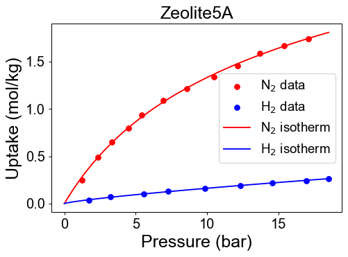
We need mixture isotherm functions to simulate PSA process. Here we define the hydrogen/nitrogen mixture isotherm functions with isofit.IAST
mix_isothrm = []
for i in range(3):
   iso_mix = lambda P,T : isof.IAST([N2_isotherm,H2_isotherm], P, T)
   mix_isothrm.append(iso_mix)
Then we need to define and run ideal PSA process.
results = []
for i in range(3):
   CI1 = simide.IdealColumn(2, mix_isothrm[i] )

   # Feed condition setting
   P_feed = 8      # Feed presure (bar)
   T_feed = 293.15    # Feed temperature (K)
   y_feed = [1/4, 3/4] # Feed mole fraction (mol/mol)
   CI1.feedcond(P_feed, T_feed, y_feed)

   # Operating condition setting
   P_high = 8 # High pressure (bar)
   P_low  = 1 # Low pressure (bar)
   CI1.opercond(P_high, P_low)

   # Simulation run
   x_tail = CI1.runideal()
   print(x_tail)       # Output: [x_H2, x_N2]
   results.append(x_tail)
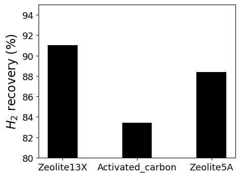
Now, we can calculate hydrogen recovery for this system. The definition of recovery is the ratio of target material between product and feed flow. The recovery is derived below.
By the assumptions of ideal PSA columns, hydrogen mole fraction in raffinate is 1 (100 mol%). Mass balance eqaution for nitrogen becomes,
Substituting above mass balance to recovery equation then,
for i in range(3):
   y_N2 = y_feed[0]
   x_N2 = results[i][0]
   R_H2 = 1- (y_N2*(1-x_N2))/(x_N2*(1-y_N2))*100
   print(f'Recovery of {Adsorbent[i]}: ', R_H2, '(%)' )
The results shows below. Finally, we found the best performance adsorbent.
2. Real PSA simulation for biogas upgrading
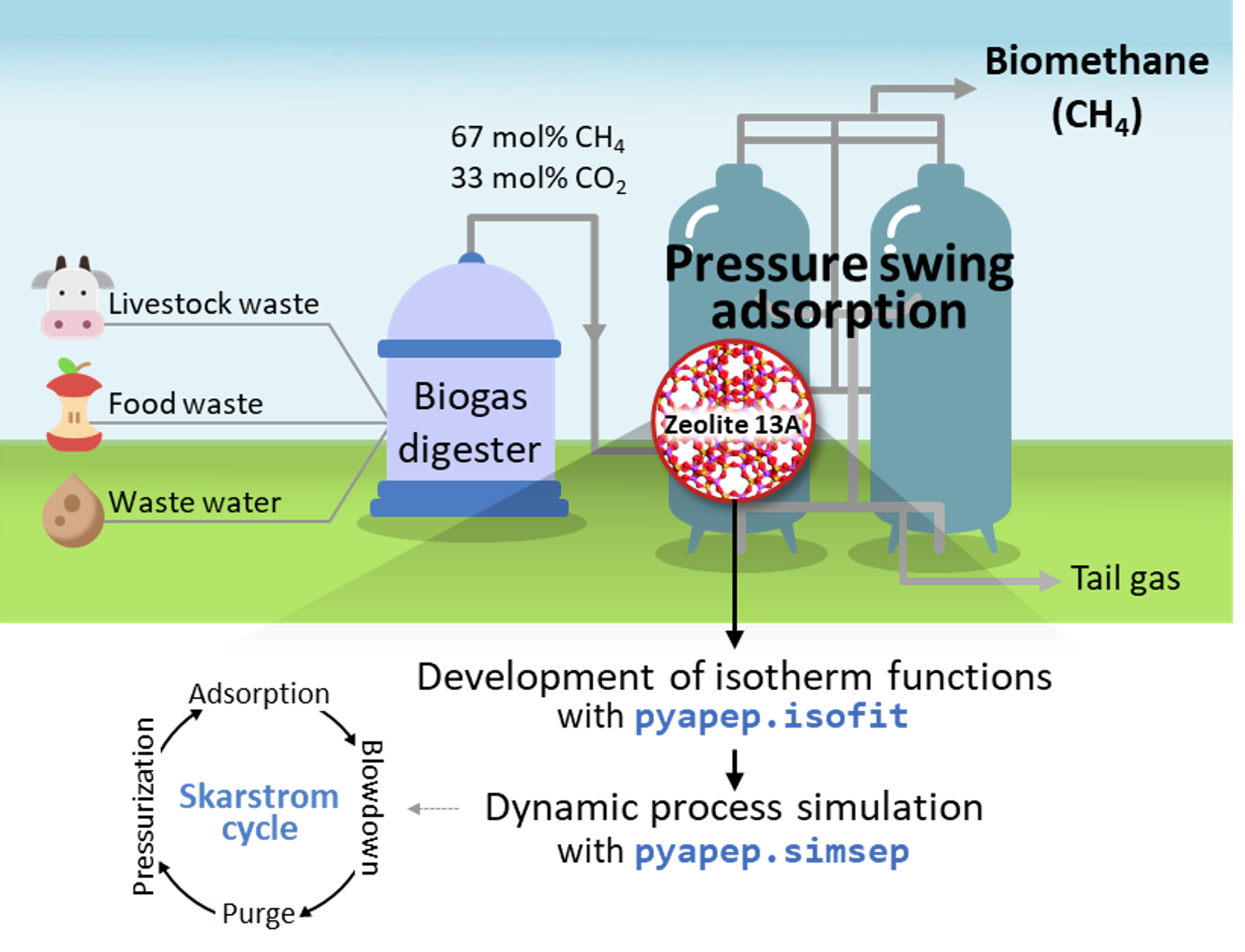
In this example, pyAPEP.simsep is used to simulate real PSA process for the separation of CO2/CH4 in biogas upgrading process.
Background
Biogas is a gas mixture that is produced when biomass such as livestock manure, agricultural waste, and sewage sludge is anaerobic digested. The composition of the biogas is generally composed of 50-70% of methane and 30-45% of carbon dioxide, and the other compositions such as H2 S, N2 , O2, and NH3 are present in a small amount of less than 4%. Methane has 21 times higher global warming potential thdan carbon dioxie, so energy recovery from biogas leads to environmental benefits as well as economic benefits, so it has recently received a lot of attention. Among the energy recovery methods, bio-mathane production through biogas upgrading is in the spotlight because the bio-mathane can be used for fuel, heating, and electricity production. Therefore, in this example, the PSA process, which is a commonly used process for biogas upgrading, is simulated using the pyAPEP.simsep module.
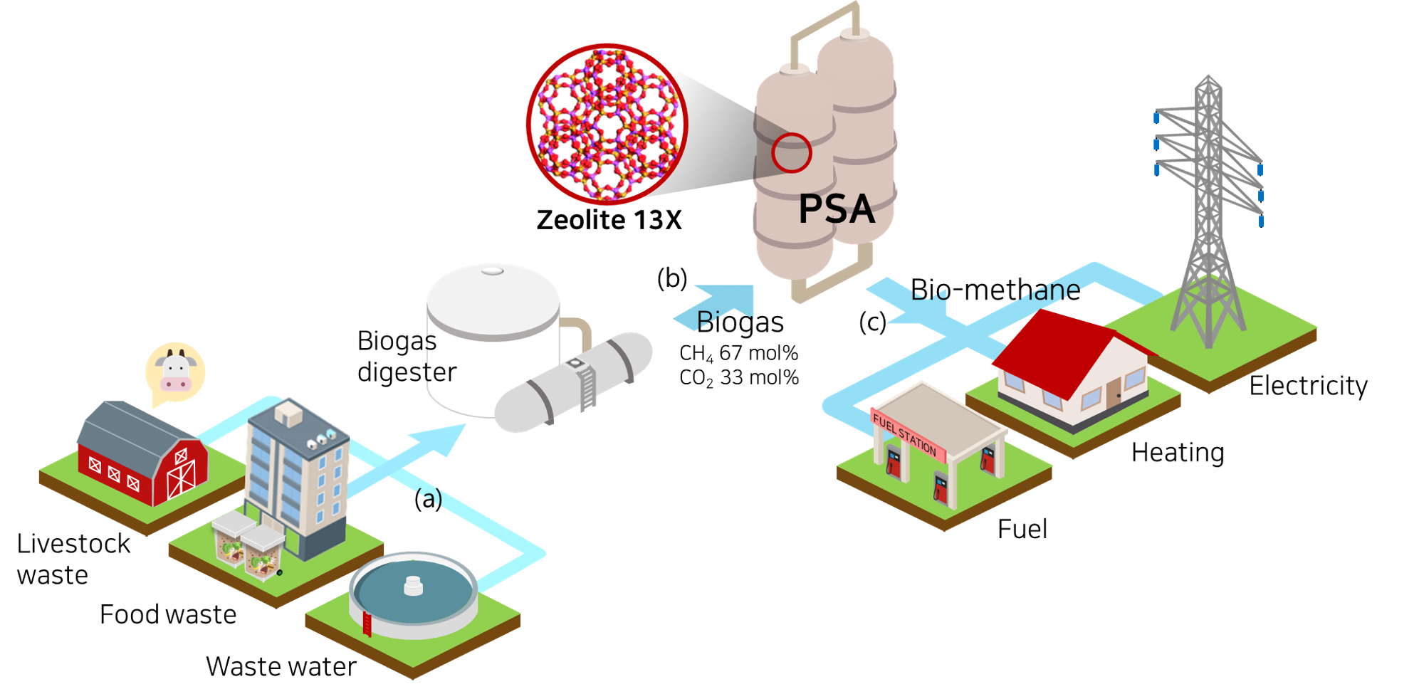
Figure. Schematic of bio-mathane production process.
Process description
Biogas produced through anaerobic digester is a gas that has a composition ratio of 67 and 33 mol% of CH4 and CO2 through a desulfurization pretreatment process. A two-component system real PSA simulation is performed based on process conditions to purify the biogas. The PSA process for biogas upgrading is adsorbed at 9 bar and desorbed at 1 bar, and the temperature and pressure of feed flow into 323 K. Here, we evaluate the commercial adsorbent, zeolite 13X for the biogas upgading.
Goal
The goal of this example is the simulation of biogas upgrading process with commercial adsorbent. Zeolite 13X and its pressure-uptake data could be found in the literature. This example contains isotherm fitting with given data(.csv), development of mixutre isotherm function and real PSA simulation.
Before we start, import pyAPEP packages. Also, users need to download adsorption data file (Example2_Zeolite13X.csv)
# pyAPEP package import
import pyadserver.isofit as isofit
import pyadserver.simsep as simsep

# Data treatment package import
import numpy as np
import pandas as pd

# Data visualization package import
import matplotlib.pyplot as plt
First, from the adsorption data samples, we need to find pure isotherm function for methane and carbon dioxide. Before developing isotherm, users need to define or import datasets. If the isotherm parameters already exist, users can use those parameters by defining isotherm function manually. Also, in this example, the single isotherm functions are used to simplify the process model.
# Data import
Data = pd.read_csv('Example2_Zeolite13X.csv')

# Pure isotherm definition
P_CO2 = Data['Pressure_CO2 (bar)'].dropna().values
q_CO2 = Data['Uptake_CO2 (mol/kg)'].dropna().values

P_CH4 = Data['Pressure_CH4 (bar)'].dropna().values
q_CH4 = Data['Uptake_CH4 (mol/kg)'].dropna().values

CO2_iso, _, _, _ = isofit.best_isomodel(P_CO2, q_CO2)
CH4_iso, _, _, _ = isofit.best_isomodel(P_CH4, q_CH4)
CO2_iso_ = lambda P,T: CO2_iso(P)
CH4_iso_ = lambda P,T: CH4_iso(P)

def MixIso(P, T):
   q1 = CO2_iso(P[0])
   q2 = CH4_iso(P[1])
   return q1, q2
Next, define and run a real PSA process. Most of the process parameters are the same as in the literature (ref). In this example, Skarstrom cycle which is the operation method for PSA process is simulated in four stages of adsorption-blowdown-purge-pressurization.
# Column design
N = 11
L = 1.35
A_cros = np.pi*0.15**2
CR1 = simsep.column(L, A_cros, n_component=2, N_node = N)

# Adsorbent parameters setting
voidfrac = 0.37      # (m^3/m^3)
D_particle = 12e-4   # (m)
rho = 1324           # (kg/m^3)
CR1.adsorbent_info(mix_iso_arr, voidfrac, D_particle, rho)

# Feed condition setting
Mmol = [0.044, 0.016]            # kg/mol
mu_visco= [11.86E-6, 16.13E-6]   # (Pa sec)
CR1.gas_prop_info(Mmol, mu_visco)

# Mass transfer information setting
k_MTC  = [1E-2, 1E-2]     # m/sec
a_surf = 1                # m2/m3
D_disp = [1E-2, 1E-2]     # m^2/sec
CR1.mass_trans_info(k_MTC, a_surf, D_disp)

# Thermal information setting
dH_ads = [31.164e3,20.856e3]   # J/mol
Cp_s = 900
Cp_g = [38.236, 35.8]          # J/mol/K
h_heat = 100                   # J/m2/K/s
CR1.thermal_info(dH_ads, Cp_s, Cp_g, h_heat)

# Boundary condition setting
P_inlet = 9.5
P_outlet = 9
T_feed = 323
y_feed = [0.67,0.33]

Cv_inlet = 0.02E-1             # inlet valve constant (m/sec/bar)
Cv_outlet= 2.0E-1           # outlet valve constant (m/sec/bar)
Q_feed = 0.05*A_cros  # volumetric flowrate (m^3/sec)

CR1.boundaryC_info(P_outlet, P_inlet, T_feed, y_feed,
                  Cv_inlet, Cv_outlet,
                  Q_inlet = Q_feed,
                  assigned_v_option = True)

# Initial condition setting
P_init = 9.25*np.ones(N)                   # (bar)
y_init = [0.001*np.ones(N), 0.999*np.ones(N)] # (mol/mol)
T_init = T_feed*np.ones(N)
q_init = mix_iso_arr(P_init*np.array(y_init), T_init)

CR1.initialC_info(P_init, T_init, T_init, y_init, q_init)
print(CR1)
This example considers the mass, momentum, and energy balance equations, therefore run_mamoen function is used to run the simulation.
# Simulation run
y_res, z_res, t_res = CR1.run_mamoen(25,n_sec = 20,
                                 CPUtime_print = True)
The simulation of the adsorption step is completed. The final results of this stage would become the initial condition of the next step, the purge step, and the boundary condition should be modified. Repeat the initial condition update, modification of boundary conditions, and the simulation running until the last step, the pressurization step.
### Blowdown step ###
CR1.next_init()
CR1.change_init_node(11)

### Operating conditions
P_inlet = 9
P_outlet = 1
T_feed = 323
y_feed = [0.001,0.999]

Cv_inlet = 0E-1             # inlet valve constant (m/sec/bar)
Cv_outlet= 1E-1           # outlet valve constant (m/sec/bar)

CR1.boundaryC_info(P_outlet, P_inlet, T_feed, y_feed,
                  Cv_inlet, Cv_outlet,
                  foward_flow_direction = False)

y_res = CR1.run_mamoen(1000,n_sec = 10, CPUtime_print = True)
### Purge step ###
CR1.next_init()

### Operating conditions
P_inlet = 1.5
P_outlet = 1
T_feed = 323
y_feed = [0.001,0.999]

Cv_inlet = 1E-1             # inlet valve constant (m/sec/bar)
Cv_outlet= 4E-1           # outlet valve constant (m/sec/bar)

CR1.boundaryC_info(P_outlet, P_inlet, T_feed, y_feed,
                  Cv_inlet, Cv_outlet,
                  foward_flow_direction = False)

y_res = CR1.run_mamoen(1000,n_sec = 10, CPUtime_print = True)
To calculate the pressurization step, an iterative method is needed to stabilize the simulation. By using the iterative calculation, the column is pressurized from 1 bar to over 8 bar.
### Pressurization step ###
CR1.next_init()

total_y = []
R_gas = 8.3145      # 8.3145 J/mol/K
P_outlet = 1
P_inlet = 2
Cv_outlet= 0E-1
T_feed = 323
y_feed = [0.33,0.67]
while P_outlet<8.1:
   Cv_inlet =(P_inlet-P_outlet)*0.1
   CR1.boundaryC_info(P_outlet, P_inlet, T_feed, y_feed,
                  Cv_inlet, Cv_outlet,
                  foward_flow_direction = True)
   y_res = CR1.run_mamoen(5,n_sec = 10, CPUtime_print = True)
   total_y.append(y_res)

   P = np.zeros(11)
   for ii in range(2):
      Tg_res = y_res[0][:,2*2*11 : 2*2*11+11]
      P = P + y_res[0][:,(ii)*11:(ii+1)*11]*R_gas*Tg_res/1E5

   P_outlet = np.mean(P[-1])
   P_inlet = P_outlet+1.1
   CR1.next_init()
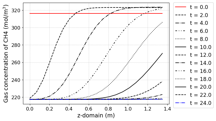
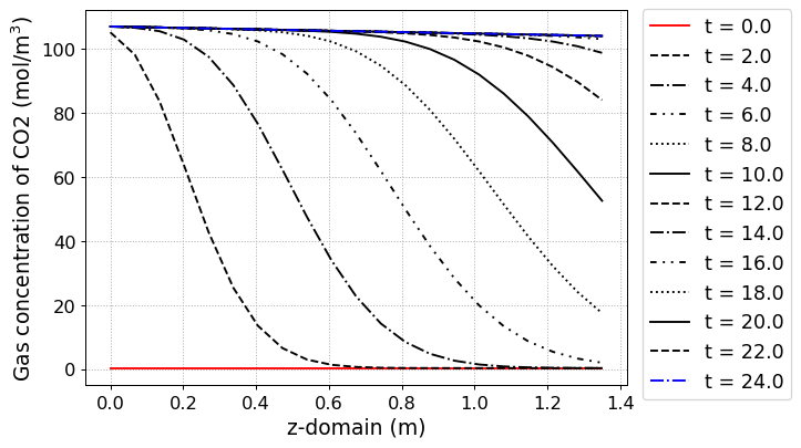
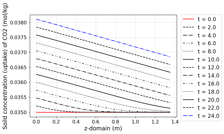
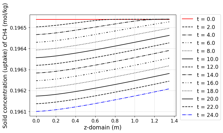
The simulation results at each step are shown in below figure.
pyAPEP.simsep module gives various results plotting functions. Here, we using those functions.
# Concentration of gas phase in z direction
fig = CR1.Graph(2, 0, loc=[1.15,0.9],
               yaxis_label = 'Gas concentration of CO2 (mol/m$^3$)',
               file_name = 'CO2_gas_conc.png')
fig = CR1.Graph(2, 1, loc=[1.15,0.9],
               yaxis_label = 'Gas concentration of CH4 (mol/m$^3$)',
               file_name = 'CH4_gas_conc.png')
# Concentration of solid phase in z direction
fig = CR1.Graph(2, 2, loc=[1.15,0.9],
               yaxis_label = 'Soild concentration (uptake) of CO2 (mol/kg)',
               file_name = 'CO2_uptake.png')
fig = CR1.Graph(2, 3, loc=[1.15,0.9],
               yaxis_label = 'Soild concentration (uptake) of CH4 (mol/kg)',
               file_name = 'CH4_uptake.png')
# Breakthrough test results
bt = CR1.breakthrough(True)
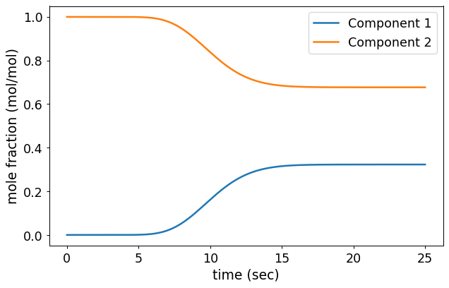
Figure. The result of breakthrough test
# Internal pressure in z direction
fig, ax = CR1.Graph_P(2, loc=[1.15,0.9])
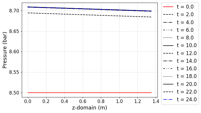
Figure. Pressure gradient with time and position
